Mapping oil production by country in R

This week, here’s another map.

As I’ve mentioned, projects like this – a few hundred lines of code, with a variety of functions from the tidyverse – are excellent practice for intermediate data scientists.

But if you’re a beginner, don’t be intimidated. You can actually learn these tools much faster than you think.

To get to a point where you really know how this works, you’ll need a few things. You will need to know a few things about ggplot2, dplyr and the tidyverse. I recommend that you break this down, line by line. Do you know all of the functions? Do you know how it all works? If you don’t, you might have some more practice to do.

Ultimately, to be “fluent” in data science in R, you should be able to write this code (or something like it) from scratch, more or less from memory.

In any case, there’s a lot going on in this code.

In a separate post, I will explain a few details about how this works, and expand on it somewhat.

In the meantime, if you want to learn to do projects like this, go through the code below. Break it down into small pieces that you can study and practice.

And if you want to know more about data visualization and data science in R, sign up for our email list.

Sign up now, and discover how to rapidly master data science

To master data visualization and data science, you need to master the essential tools.

Moreover, to make rapid progress, you need to know what to learn, what not to learn, and you need to know how to practice what you learn.

Sharp Sight is dedicated to teaching you how to master the tools of data science as quickly as possible.

Sign up now for our email list, and you’ll receive regular tutorials and lessons.

You’ll learn:

• How to do data visualization in R
• How to practice data science
• How to apply data visualization to more advanced topics (like machine learning)
• … and more

If you sign up for our email list right now, you’ll also get access to our “Data Science Crash Course” for free.

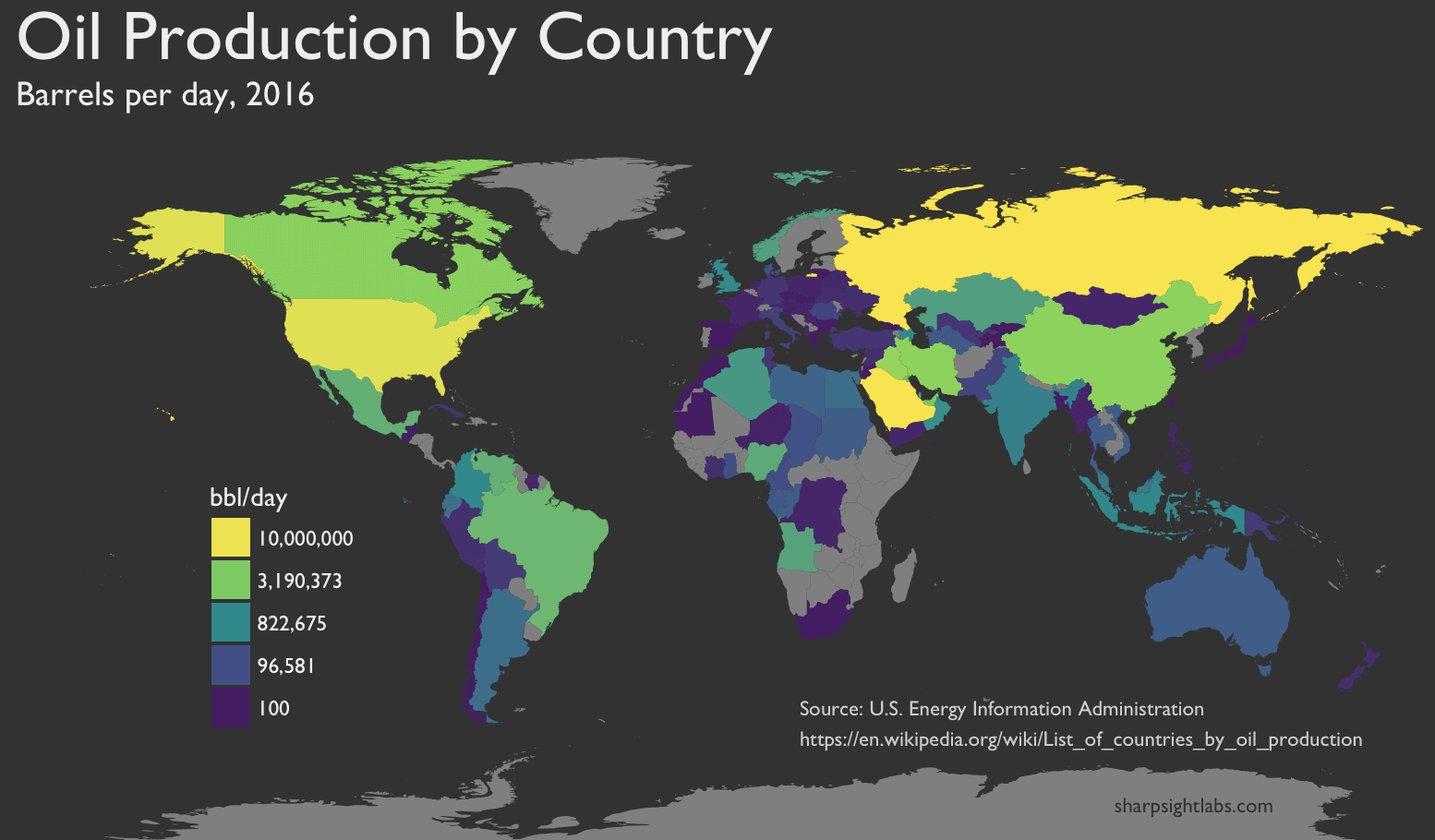
Code: mapping oil production by country

#==============
# LOAD PACKAGES
#==============

library(tidyverse)
library(sf)
library(rvest)
library(stringr)
library(scales)
#library(viridis)



#============
# SCRAPE DATA
#============

df.oil <- read_html("https://en.wikipedia.org/wiki/List_of_countries_by_oil_production") %>%
  html_nodes("table") %>%
  .[[1]] %>%
  html_table()



#====================
# CHANGE COLUMN NAMES 
#====================

colnames(df.oil) <- c('rank', 'country', 'oil_bbl_per_day')



#=============================
# WRANGLE VARIABLES INTO SHAPE
#=============================


#----------------------------------
# COERCE 'rank' VARIABLE TO INTEGER
#----------------------------------

df.oil <- df.oil %>% mutate(rank = as.integer(rank)) 

df.oil %>% glimpse()



#---------------------------------------------------
# WRANGLE FROM CHARACTER TO NUMERIC: oil_bbl_per_day
#---------------------------------------------------

df.oil <- df.oil %>% mutate(oil_bbl_per_day = oil_bbl_per_day %>% str_replace_all(',','') %>% as.integer())


# inspect
df.oil %>% glimpse()


#===========================
#CREATE VARIABLE: 'opec_ind'
#===========================

df.oil <- df.oil %>% mutate(opec_ind = if_else(str_detect(country, 'OPEC'), 1, 0))


#=========================================================
# CLEAN UP 'country'
# - some country names are tagged as being OPEC countries
#   and this information is in the country name
# - we will strip this information out
#=========================================================

df.oil <- df.oil %>% mutate(country = country %>% str_replace(' \\(OPEC\\)', '') %>% str_replace('\\s{2,}',' '))


# inspect
df.oil %>% glimpse()


#------------------------------------------
# EXAMINE OPEC COUNTRIES
# - here, we'll just visually inspect
#   to make sure that the names are correct
#------------------------------------------

df.oil %>% 
  filter(opec_ind == 1) %>%
  select(country)



#==================
# REORDER VARIABLES
#==================

df.oil <- df.oil %>% select(rank, country, opec_ind, oil_bbl_per_day)

df.oil %>% glimpse()



#========
# GET MAP
#========

map.world <- map_data('world')

df.oil


#==========================
# CHECK FOR JOIN MISMATCHES
#==========================

anti_join(df.oil, map.world, by = c('country' = 'region'))


# rank                           country opec_ind oil_bbl_per_day
# 1   67 Congo, Democratic Republic of the        0          20,000
# 2   47               Trinidad and Tobago        0          60,090
# 3   34            Sudan and  South Sudan        0         255,000
# 4   30            Congo, Republic of the        0         308,363
# 5   20                    United Kingdom        0         939,760
# 6    3                     United States        0       8,875,817



#=====================
# RECODE COUNTRY NAMES
#=====================

map.world %>%
  group_by(region) %>%
  summarise() %>%
  print(n = Inf)


# UK
# USA
# Democratic Republic of the Congo
# Trinidad
# Sudan
# South Sudan


df.oil <- df.oil %>%  mutate(country = recode(country, `United States` = 'USA'
                                 , `United Kingdom` = 'UK'
                                 , `Congo, Democratic Republic of the` = 'Democratic Republic of the Congo'
                                 , `Trinidad and Tobago` = 'Trinidad'
                                 , `Sudan and South Sudan` = 'Sudan'
                                 #, `Sudan and  South Sudan` = 'South Sudan'
                                 , `Congo, Republic of the` = 'Republic of Congo'
                                 )
                   )



#-----------------------
# JOIN DATASETS TOGETHER
#-----------------------

map.oil <- left_join( map.world, df.oil, by = c('region' = 'country')) 



#=====
# PLOT
#=====

# BASIC (this is a first draft)

ggplot(map.oil, aes( x = long, y = lat, group = group )) +
  geom_polygon(aes(fill = oil_bbl_per_day))



#=======================
# FINAL, FORMATTED DRAFT
#=======================


df.oil %>% filter(oil_bbl_per_day > 822675) %>% summarise(mean(oil_bbl_per_day))
# 3190373

df.oil %>% filter(oil_bbl_per_day < 822675) %>% summarise(mean(oil_bbl_per_day))
# 96581.08



ggplot(map.oil, aes( x = long, y = lat, group = group )) +
  geom_polygon(aes(fill = oil_bbl_per_day)) +
  scale_fill_gradientn(colours = c('#461863','#404E88','#2A8A8C','#7FD157','#F9E53F')
                       ,values = scales::rescale(c(100,96581,822675,3190373,10000000))
                       ,labels = comma
                       ,breaks = c(100,96581,822675,3190373,10000000)
                       ) +
  guides(fill = guide_legend(reverse = T)) +
  labs(fill = 'bbl/day'
       ,title = 'Oil Production by Country'
       ,subtitle = 'Barrels per day, 2016'
       ,x = NULL
       ,y = NULL) +
  theme(text = element_text(family = 'Gill Sans', color = '#EEEEEE')
        ,plot.title = element_text(size = 28)
        ,plot.subtitle = element_text(size = 14)
        ,axis.ticks = element_blank()
        ,axis.text = element_blank()
        ,panel.grid = element_blank()
        ,panel.background = element_rect(fill = '#333333')
        ,plot.background = element_rect(fill = '#333333')
        ,legend.position = c(.18,.36)
        ,legend.background = element_blank()
        ,legend.key = element_blank()
        ) +
  annotate(geom = 'text'
           ,label = 'Source: U.S. Energy Information Administration\nhttps://en.wikipedia.org/wiki/List_of_countries_by_oil_production'
           ,x = 18, y = -55
           ,size = 3
           ,family = 'Gill Sans'
           ,color = '#CCCCCC'
           ,hjust = 'left'
           )

And here’s the finalized map that the code produces:

To get more tutorials that explain how this code works, sign up for our email list.